
Electrolytic solutions are those that are capable of conducting an electric current. A substance that, when added to water, renders it conductive, is known as an electrolyte. A common example of an electrolyte is ordinary salt, sodium chloride. Solid NaCl and pure water are both non-conductive, but a solution of salt in water is readily conductive. A solution of sugar in water, by contrast, is incapable of conducting a current; sugar is therefore a non-electrolyte.
These facts have been known since 1800 when it was discovered that an electric current can decompose the water in an electrolytic solution into its elements (a process known as electrolysis). By mid-century, Michael Faraday had made the first systematic study of electrolytic solutions.
Faraday recognized that in order for a sample of matter to conduct electricity, two requirements must be met:
- The matter must be composed of, or contain, electrically charged particles.
- These particles must be mobile; that is, they must be free to move under the influence of an external applied electric field.
In metallic solids, the charge carriers are electrons rather than ions; their mobility is a consequence of the quantum-mechanical uncertainty principle which promotes the escape of the electrons from the confines of their local atomic environment.
In the case of electrolytic solutions, Faraday called the charge carriers ions (after the Greek word for "wanderer"). His most important finding was that each kind of ion (which he regarded as an electrically-charged atom) carries a definite amount of charge, most commonly in the range of ±1-3 units.
The fact that the smallest charges observed had magnitudes of ±1 unit suggested an "atomic" nature for electricity itself, and led in 1891 to the concept of the "electron" as the unit of electric charge — although the identification of this unit charge with the particle we now know as the electron was not made until 1897.
← An ionic solid such as NaCl is composed of charged particles, but these are held so tightly in the crystal lattice that they are unable to move about, so the second requirement mentioned above is not met and solid salt is not a conductor. If the salt is melted or dissolved in water, the ions can move freely and the molten liquid or the solution becomes a conductor.
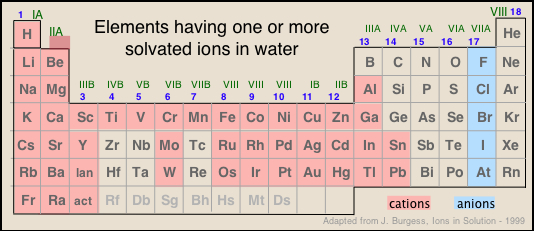
Since positively-charged ions are attracted to a negative electrode that is traditionally known as the cathode, these are often referred to as cations. Similarly, negatively-charged ions, being attracted to the positive electrode, or anode, are called anions. (These terms were all coined by Faraday.)
Why water is such a good solvent for ions
Although we tend to think of the solvent (usually water) as a purely passive medium within which ions drift around, it is important to understand that
- Electrolytic solutions would not exist without the active involvement of the solvent in reducing the strong attractive forces that hold solid salts and molecules such as HCl together;
- Once the ions are released, they are stabilized by interactions with the solvent molecules.
Water is not the only liquid capable of forming electrolytic solutions, but it is by far the most important. It is therefore essential to understand those properties of water that influence the stability of ions in aqueous solution.
Water's large dielectric constant suppresses ionic attractions
According to Coulomb's law, the force between two charged particles is directly proportional to the product of the two charges, and inversely proportional to the square of the distance between them:
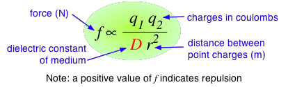
The proportionality constant D is the dimensionless dielectric constant. Its value in empty space is unity, but in other media it will be larger. Since D appears in the denominator, this means that the force between two charged particles within a gas or liquid will be less than if the particles were in a vacuum.
Water has one of the highest dielectric constants of any known liquid; the exact value varies with the temperature, but 80 is a good round number to remember. When two oppositely-charged ions are immersed in water, the force acting between them is only 1/80 as great as it would be between the two gaseous ions at the same distance.
It can be shown that in order to separate one mole of Na+ and Cl– ions at their normal distance of 23.6 pm in solid sodium chloride, the work required will be 586 J in a vacuum, but only 7.3 J in water
The dielectric constant, by the way, is a bulk property of matter, rather than being a property of the molecule itself, as is the dipole moment. It is a cooperative effect of all the molecules in the liquid, and is a measure of the extent to which an applied electric field will cause the molecules to line up with the negative ends of their dipoles pointing toward the positive direction of the electric field. The high dielectric constant of water is a consequence of the small size of the H2O molecule in relation to its large dipole moment.
When one molecule is reoriented by the action of an external electric field, local hydrogen bonding tends to pull neighboring molecules into the same alignment, thus producing an additive effect that would be absent if the molecules were all acting independently.
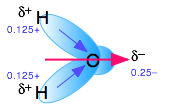
Water's dipole moment stabilizes dissolved ions through hydrogen bonding
When an ion is introduced into a solvent, the attractive interactions between the solvent molecules must be disrupted in order to create space for the ion. This costs energy and would by itself tend to inhibit dissolution. But if the solvent has a high permanent dipole moment, the energy cost is more than recouped by the ion-dipole attractions between the ion and the surrounding solvent molecules.
Water is not the only electrolytic solvent
... but it is by far the best. For some purposes, chemists occasionally need to employ non-aqueous solvents when studying electrolytes. Here are a few examples:
| solvent | bp, °C | fp, °C | D | dipole moment | specific conductivity, cm |
|---|---|---|---|---|---|
| water | 0 | 100 | 78.4 | 1.87 | 5.5 × 10⁻⁹ |
| methanol | 64.7 | –98 | 32.7 | 2.87 | 1.5 × 10⁻⁹ |
| ethanol | 78.3 | –114 | 24.5 | 1.66 | 1.35 × 10⁻⁹ |
| acetonitrile | 81.6 | –43.8 | 37.5 | 3.4 | 6 × 10⁻¹⁰ |
| dimethyl sulfoxide | 189 | 18.5 | 46.7 | 3.9 | 2 × 10⁻⁹ |
| ethylene carbonate | 238 | 36.4 | 89.6 | 4.87 | < 1 × 10⁻⁹ |
The kinds of ions we will consider in this lesson are mostly those found in solutions of common acids or salts. As is evident from the image below, most of the metallic elements form monatomic cations, but the number of monatomic anions is much smaller. This reflects the fact that many single-atom anions such as hydride H–, oxide O2–, sulfide S2– and those in Groups 15 and 16, are unstable in (i.e., react with) water, and their major forms are those in which they are combined with other elements, particularly oxygen. Some of the more familiar oxyanions are hydroxide OH–, carbonate CO32–, nitrate NO3–, sulfate SO42–, chlorate ClO42–, and arsenate AsO42–.
Dissolved ions disrupt water structure
Pure water is believed to consist of ever-changing regions of hydrogen-bonded molecules loosely organized into irregular ice-like tetrahedral "clusters", interspersed with more dense regions of jumbled H2O molecules in which hydrogen bonding still occurs but not to the extent that it controls the local structure. Clusters are estimated to contain 50-200 H2O molecules at room temperature and to have lifetimes in the range of 10-100 picoseconds.
Individual hydrogen bonds have lifetimes of only a few picoseconds, so even within a cluster, these bonds are continually breaking and re-forming in new configurations. It is believed that when one bond breaks, it initiates a cascade of breaks among nearby bonds as these molecules settle into more stable tetrahedral arrangements.
There is probably a continual migration of individual H2O molecules between clustered and disordered regions. As the temperature rises, the more disordered regions begin to grow at the expense of the clusters.
When an ion is introduced into water, the relatively strong ion-dipole attractions tend to impose an octahedral-like configuration on the surrounding H2O molecules, thus disrupting the quasi-tetrahedral structure of the bulk water. This can either increase or decrease the local ordering of water around the ion:
- Small ions such as Li+, Mg2+, Al+3+ and F– have high charge densities which strongly align the surrounding H2O's. The amount of new ordering thus created tends to outweigh the disorder due to the "hole" in the water structure that the ion creates. Such ions tend to pull H2O molecules from bulk water into the more compact hydration shell; they are therefore said to be "structure-making" and often exhibit negative entropies of hydration. NO3– and ClO4– are also believed to fall into this category.
- Larger and less-polarizing ions such as Cs+, Br– and I–, as well as the polyatomic ions SO42– and PO43– are less effective in aligning the surrounding H2O molecules, but their larger volumes tend to cause more local disorder. The "structure-breaking" ions commonly have positive hydration entropies.
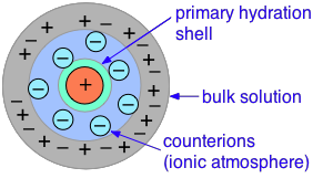
Aqueous ions are surrounded by hydration shells
As was explained in the section on the energetics of salt dissolution, the ability of salts to dissolve in water depends strongly on their stabilization by the solvent molecules. This process is known generally as solvation, and in the case of water, as hydration. All ions dissolved in water are hydrated.
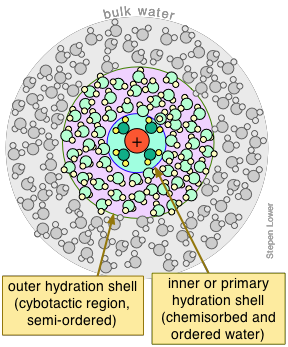
Bear in mind that the attractive forces that are operational here — hydrogen bonding (dipole-dipole) and even the stronger ion-dipole forces that bind the waters in the primary shell to the central ion — are continually subject to disruption by thermal motions. This affects even the waters within the primary shell; residence times of these H2O molecules are usually less than 10–4 sec.
Hydration numbers are generally only averages
The total number of waters bound to the central ion is known as the hydration number of the ion. Unfortunately, what we mean by "attached" is somewhat difficult to define, and experimental estimates seem to depend a lot on the particular methods employed to investigate it. Whatever the value may be at any instant, it is quite certain to be continually changing, so we can only regard hydration numbers as averages. Moreover, these H2Os are subject to replacement by other ligands that have a similar or greater affinity for the central ion.
| ion | Li+ | Na+ | K+ | Cs+ | Mg2+ | Ca2+ | Ba2+ | Zn2+ | Fe2+ | Al3+ | Cr4+ |
|---|---|---|---|---|---|---|---|---|---|---|---|
| radius, pm | 76 | 102 | 152 | 72 | 100 | 149 | 88 | 70 | 54 | 75 | |
| hyd. no. | 3-22 | 3-13 | 1-7 | 1-4 | 5-14 | 4-12 | 3-9 | 6-13 | 6-13 | 6-21 | 6-17 |
In general, there appears to be more agreement on numbers closer to the upper ends of these ranges. This supports the generally-held assumption that the smaller and more highly charged the ion (i.e., the greater its charge density), the more highly hydrated it will be.
Transition-metal complexes
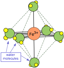
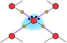
The ions formed by the transition metals (i.e., most cations!) are bound to a small number (usually four or six) H2O molecules by coordinate covalent bonds involving d-orbitals, as indicated by the example of Fe(H2O)63+, known as hexaaquairon(III). These waters comprise part of the primary hydration shell, which may also include a number of non-coordinated H2Os.
Most positive ions act as acids in water
It is generally known that aqua-complexes such as the iron-III example shown above act as acids (for details, see the section on hydrous complexes in another lesson of this series). What is less widely understood is that all cations are acidic.
The "source" of the acidity is the the primary hydration shell. The nearby positive charge on the ion M+ encourages the loss of a proton from an attached H2O according to
M(H2O)+ → M(OH)– + H+
For a more detailed discussion of cation acid strengths, see the article All Positive Ions Give Acid Solutions in Water: Stephen J. Hawkes, J Chem Educ 1996(6) 516-517. The pKa values shown in the table are taken from this article.
The acid strengths of these ions depend on their charge densities. The effect is negligible in alkali-metal salts, with the exception of those of the very small Li+ ion. In the ions of Group 2, 0.1 M L–1 solutions of the salts will reduce the pH of water by a few tenths of a unit. Ions of Group 3 and beyond can exhibit strengths comparable to that of acetic acid (pKa 4.75).
Some pKa values of 0.1 M solutions of typical ions:
| Li+ | Mg2+ | Cr3+ | Fe2+ | Fe3+ | Cu2+ | Sn2+ | Al3+ |
| 13.6 | 11.2 | 3.7 | 9.4 | 2.2 | 7.5 | 3.4 | 5.0 |
Given the above values, it is not surprising that a solution of FeCl3 is often referred to as an "acid" in industries that use it.
Some salts incorporate hydration water into their solid forms
Many of these ions bind water molecules so strongly that they remain hydrated even in their crystalline forms.
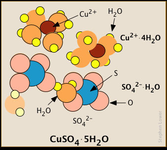
Similarly, each Al3+ ion in the double hydrate KAl(SO4)2·12H2O is surrounded by six. Some of the water molecules in these crystals are bound to specific ions, while others belong to the crystal structure as a whole.
Dissolved ions interact strongly with each other
It is of course impossible to introduce a single kind of ion into water; bulk matter cannot possess a significant net electric charge, so all ionic solutions contain both anions and cations in the proportions required to ensure electroneutrality. Coulombic interactions between charged particles fall off with separation distance far more slowly than do the weaker ion-dipole forces responsible for water ordering, and are thus operative even in solutions that we would normally regard as quite dilute — down to about 10–4 M L–1.
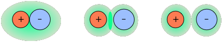
Oppositely-charged ions tend to pair up in solution
Depending on the sizes and charges of the two kind of ions, they may form relatively stable ion pairs in which the "bonding" is purely electrostatic and independent of the chemical properties of the ions.
As was mentioned in a previous lesson of this unit, neglect of ion-pairing can lead to erroneous assumptions about the concentrations of "free" ions in solutions, and misinterpretation of solubility-product calculations.
- Thus, in addition to forming the sparingly-soluble solid CdI2, part of the cadmium in a solution in equilibrium with the two ions will exist as the soluble species CdI–(aq) and CdI20(aq).
- Similarly, solutions in equilibrium with Ca(OH)2(s) will also contain CaOH+(aq) and Ca(OH)20(aq).
- The ion-pair CaCO30(aq) is believed to tie up a significant fraction of the total carbonate when water is in equilibrium with solid calcium carbonate.
The ions in the more strongly-bound pairs will be in contact and within a common hydration shell, whereas others may have only their shells in contact.
Electrostatic forces lead to local charge imbalances surrounding an ion
Ionic solutions generally exhibit non-ideal behavior
You will recall that the conceptual definition of an ideal solution requires that the interactions of solvent-solvent, solvent-solute, and solute-solute molecules are identical — something that is clearly not possible in ionic solutions. As a consequence, the operational criteria of solution ideality — linear dependence of colligative and other properties on nominal concentrations, does not apply.
For the reasons outlined in the preceding section, you cannot realistically expect calculations based on equilibrium constants to reliably predict the compositions of solutions having significant concentrations of ions.
The actual quantity we use to express the summed concentrations of ions of all kinds in a solution is the ionic strength. See this Wikipedia article for a definition and examples.
What "significant" means in this context depends on the charges of the ions, and this includes "spectator" ions that are not directly involved in a reaction. A very crude rule-of-thumb is that ion concentrations in excess of
0.0001 M L–1 are likely to exhibit non-ideal behavior.
Ionic activities and activity coefficients
The quantitative treatment of ionic solutions is based on the Debye-Hückel theory which was developed in the 1920s. This theory models the electrostatic interactions between ions and their ionic atmospheres, and can predict mean ionic activity coefficient for solutions whose ionic strengths are not very high. Many extensions to this model have been suggested; all are mathematically complicated and all fail for "really concentrated" solutions.
The practical approach to the problem of non-ideality is to introduce a quantity known as the activity, which can be thought of as the thermodynamically-effective concentration. The relation between activity a and the "analytical" concentration c is given by the activity coefficient γ (gamma):
a = γ c
- An ideal solution has an activity coefficient of unity.
- As ionic concentrations increase, activity constants diminish.
- Activity coefficients approach unity in the limit of zero concentration.
Because solutions containing ions of a single charge species cannot be prepared, all experimental measurements can only yield mean ionic activity coefficients γ±.
For reliable calculations, it is necessary to replace ordinary concentration-based equilibrium constants Kc with thermodynamically-effective equilibrium constants Ka:
Ka = γ± Kc
Basics of ionic conduction
The conduction of electricity through an ionic solution is different from metallic conduction in two fundamental ways:
- The current is associated with the transport of relatively large and massive hydrated ions, rather than by nearly weightless electrons. Electrons move largely unimpeded through the metal. But ions, with their closely-held waters of hydration and more diffuse secondary hydration shell and oppositely-charged counterions, must disrupt the local hydrogen-bonded water structure as they move through the solution.
- Transfer of electric charge into and out of the solution occurs at electrodes, and is accompanied by chemical reactions at these interfaces.
Electrolytic conduction involves the transport of electric charge in the form of hydrated ions. Movement of these ions in response to an electric potential gradient is known as migration.
Electric charge is measured in units of coulombs. A coulomb is an ampere-second; if a current of 1 amp flows for one minute, the quantity of charge transported will be 3600 C.
When charges migrate in an electric field, thermodynamic work is done. One C of charge moving through a potential difference of one volt results in the performance of one joule of work.
Electrical resistance, conductance, and conductivity
Ionic migration is always impeded by the drag created by the hydration shell as the ions break their way through the hydrogen-bonded water structure. Electrolytic conduction is therefore always associated with a certain amount of electrical resistance. Electrical resistance is defined by Ohm's law R = V/i in which V is the potential difference (voltage) and i is the current. Resistance is expressed in ohms, whose symbol is Ω (omega).
Resistance is an extensive property because it depends on the thickness and cross-section area of the material through which the current flows. The intensive analog of resistance is the resistivity ρ (rho), defined as the resistance between opposite faces of a 1-cm cube. Resistivity is usually expressed in ohm-cm.
In working with electrolytic solutions, it is more convenient to use the corresponding reciprocal properties:
conductance Λ (lambda) = 1/R
conductivity κ (kappa) = 1/ρ
The SI unit of conductance is the siemens, indicated by the symbol S.
Conductivity, the reciprocal of the resistivity, is frequently expressed in ohm–1 cm–1
or S cm–1, but the SI units are S m–1.
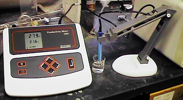
Conductance measurements
The traditional method of measuring resistance or conductance is by means of a Wheatstone bridge arrangement in which a known resistance is balanced against the unknown resistance. The latter consists of a conductivity cell having electrodes of fixed size and spacing. Nowadays it is more common to employ a digital measuring device.
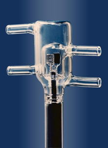
In practical measurements of conductivity, no attempt is made to define the precise dimensions of the conductive path. Instead, the conductance cell is first calibrated by filling it with a standardized solution of potassium chloride, for which extensive conductivity data is available.
Because resistances can be measured to very high precision, conductance measurements can be extended to very dilute solutions if impurities are guarded against, of which dissolved atmospheric CO2 is the most common.
Heroic measures may be required to purify water sufficiently: after 42 successive vacuum distillations, Kohlrausch in 1894 obtained a "conductivity water" with κ = 0.043 × 10⁻⁶ S cm–1 at 18°C. Ordinary distilled water in equilibrium with atmospheric CO2 has a conductivity that is 16 times greater.
It is now known that ordinary distillation cannot entirely remove all impurities from water. Ionic impurities get entrained into the fog created by breaking bubbles and are carried over into the distillate by capillary flow along the walls of the apparatus. Organic materials tend to be steam-volatile ("steam-distilled").
The best current practice is to employ a special still made of fused silica in which the water is volatilized from its surface without boiling. Complete removal of organic materials is accomplished by passing the water vapor through a column packed with platinum gauze heated to around 800°C through which pure oxygen gas is passed to ensure complete oxidation of carbon compounds.
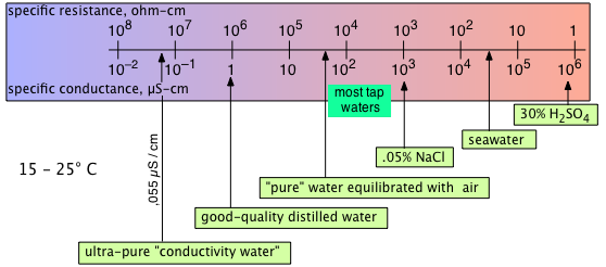
Conductance measurements are widely used to gauge water quality, especially in industrial settings in which concentrations of dissolved solids must be monitored in order to schedule maintenance of boilers and cooling towers.
Molar and equivalent conductivity
The conductance of a solution depends on 1) the concentration of the ions it contains, 2) on the number of charges carried by each ion, and 3) on the mobilities of these ions. The latter term refers to the ability of the ion to make its way through the solution, either by ordinary thermal diffusion or in response to an electric potential gradient.
The first step in comparing the conductances of different solutes is to reduce them to a common concentration. For this, we define the conductance per unit concentration which is known as the molar conductivity, denoted by the upper-case Greek lambda:
Λ = κ/c
When κ is expressed in S cm–1, C should be in mol cm–3, so Λ will have the units S cm2. This is best visualized as the conductance of a cell having 1-cm2 electrodes spaced 1 cm apart — that is, of a 1 cm cube of solution. But because chemists generally prefer to express concentrations in mol L–1 or
mol dm–3 (mol/1000 cm3) , it is common to write the expression for molar conductivity as
Λ = 1000κ/c
whose units are S cm2 mol L–1. This corresponds to a 1000 cm–3 cube of solution composed of two 1000-cm2 electrodes, separated again by 1 cm.
But if c is the concentration in moles per liter, this will still not fairly compare two salts having different stoichiometries, such as AgNO3 and FeCl3, for example. If we assume that both salts dissociate completely in solution, each mole of AgNO3 yields two moles of charges, while FeCl3 releases six(i.e., one Fe3+ ion, and three Cl– ions.) So if one neglects the [rather small] differences in the ionic mobilities, the molar conductivity of FeCl3 would be three times that of AgNO3.
Equivalents and equivalent concentration
The most obvious way of getting around this is to note that one mole of a 1:1 salt such as AgNO3 is "equivalent" (in this sense) to 1/3 of a mole of FeCl3, and of ½ a mole of MgBr2.
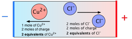
To find the number of equivalents that correspond a given quantity of a salt, just divide the number of moles by the total number of positive charges in the formula unit. (If you like, you can divide by the number of negative charges instead; because these substances are electrically neutral, the numbers will be identical.)
Note that we can refer to equivalent concentrations of individual ions as well as of neutral salts. Also, since acids can be regarded as salts of H+, we can apply the concept to them; thus a 1M L–1 solution of sulfuric acid H2SO4 has a concentration of
2 eq L–1.
The following diagram summarizes the relation between moles and equivalents for CuCl2:
Equivalent conductivity
The concept of equivalent concentration allows us to compare the conductances of different salts in a meaningful way. Equivalent conductivity is defined similarly to molar conductivity
Λ = κ/c
except that the concentration term is now expressed in equivalents per liter instead of moles per liter. (In other words, the equivalent conductivity of an electrolyte is the conductance per equivalent per liter.)
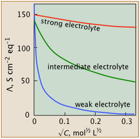
These studies revealed that the equivalent conductivities of electrolytes all diminish with concentration (or more accurately, with the square root of the concentration), but they do so in several distinct ways that are distinguished by their behaviors at very small concentrations. This led to the classification of electrolytes as weak, intermediate, and strong.
 Strong electrolytes
- These well-behaved systems include many simple salts such as NaCl, as well as all strong acids.
The Λ vs. √c plots closely follow the linear relation - Λ = Λ° – b √c
- Intermediate electrolytes
- These "not-so-strong" salts can't quite conform to the linear equation above, but their conductivities can be extrapolated to infinite dilution.
- Weak electrolytes
- "Less is more" for these oddities which possess the remarkable ability to exhibit infinite equivalent conductivity at infinite dilution. Although Λ° cannot be estimated by extrapolation, there is a clever work-around.
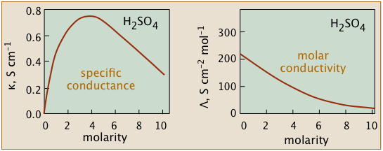
Conductivity diminishes as concentrations increase
Since ions are the charge carriers, we might expect the conductivity of a solution to be directly proportional to their concentrations in the solution. So if the electrolyte is totally dissociated, the conductivity should be directly proportional to the electrolyte concentration.
But this ideal behavior is never observed; instead, the conductivity of electrolytes of all kinds diminishes as the concentration rises.
The non-ideality of electrolytic solutions is also reflected in their colligative properties, especially freezing-point depression and osmotic pressure.
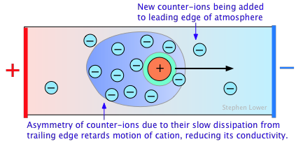
The primary cause of this is the presence of the ionic atmosphere that was introduced above. To the extent that ions having opposite charge signs are more likely to be closer together, we would expect their charges to partially cancel, reducing their tendency to migrate in response to an applied potential gradient.
A secondary effect arises from the fact that as an ion migrates through the solution, its counter-ion cloud does not keep up with it. Instead, new counter-ions are continually acquired on the leading edge of the motion, while existing ones are left behind on the opposite side. It takes some time for the lost counter-ions to dissipate, so there are always more counter-ions on the trailing edge. The resulting asymmetry of the counter-ion field exerts a retarding effect on the central ion, reducing its rate of migration, and thus its contribution to the conductivity of the solution.
The quantitative treatment of these effects was first worked out by P. Debye and W. Huckel in the early 1920's, and was improved upon by Ostwald a few years later. This work represented one of the major advances in physical chemistry in the first half of the 20th Century, and put the behavior of electrolytic solutions on a sound theoretical basis. Even so, the D-H theory breaks down for concentrations in excess of about 10–3 M L–1 for most ions.
Many electrolytes are not totally dissociated in solution
The nearly-linear nature of conductivity-vs.-√c plots for strong electrolytes is largely explained by the effects discussed immediately above. The existence of intermediate electrolytes served as the first indication that many salts are not completely ionized in water; this was soon confirmed by measurements of their colligative properties.
The curvature of the plots for intermediate electrolytes is a simple consequence of the LeChâtelier effect, which predicts that the equilibrium
MX(aq) = M+(aq) + X–(aq)
will shift to the left as the concentration of the "free" ions increases. In more dilute solutions, the actual concentrations of these ions is smaller, but their fractional abundance in relation to the undissociated form is greater. As the solution approaches zero concentration, virtually all of the MX(aq) becomes dissociated, and the conductivity reaches its limiting value.
Weak electrolytes are dissociated only at extremely high dilution
| hydrofluoric acid | HF | Ka = 10–3.2 |
| acetic acid | CH3COOH | Ka = 10–6.3 |
| bicarbonate ion | HCO3– | Ka = 10–10.3 |
| ammonia | NH3 | Kb = 10–4.7 |
These weak electrolytes, like the intermediate ones, will be totally dissociated at the limit of zero concentration; if the scale of the weak-electrolyte plot (blue) shown above were magnified by many orders of magnitude, the curve would resemble that for the intermediate electrolyte above it, and a value for Λ° could be found by extrapolation. But at such a high dilution, the conductivity would be so minute that it would be masked by that of water itself (that is, by the H+ and OH– ions in equilibrium with the massive 55.6 M L–1 concentration of water) — making values of Λ in this region virtually unmeasurable.
The motion of ions in solution is mainly random
The conductance of an electrolytic solution results from the movement of the ions it contains as they migrate toward the appropriate electrodes. But the picture we tend to have in our minds of these ions moving in a orderly, direct march toward an electrode is wildly mistaken.
Remember: The thermally-induced random motions of molecules is known as diffusion.
The term migration refers specifically to the movement of ions due to an externally-applied electrostatic field.
The average thermal energy at temperatures within water's liquid range (given by RT ) is sufficiently large to dominate the movement of ions even in the presence of an applied electric field. This means that the ions, together with the water molecules surrounding them, are engaged in a wild dance as they are buffeted about by thermal motions (which include Brownian motion).
If we now apply an external electric field to the solution, the chaotic motion of each ion is supplemented by an occasional jump in the direction dictated by the interaction between the ionic charge and the field. But this is really a surprisingly tiny effect:
It can be shown (we will spare you the math!) that in a typical electric field of 1 volt/cm, a given ion will experience only about one field-directed
(non-random) jump for every 105 random jumps.
This translates into an average migration velocity of roughly 10–7 m sec–1
(10–4 mm sec–1). Given that the radius of the H2O molecule is close to
10–10 m, it follows that about 1000 such jumps are required to advance beyond a single solvent molecule!
Ions migrate independently during electrolysis
All ionic solutions contain at least two kinds of ions (a cation and an anion), but may contain others as well. In the late 1870's, the physicist Friedrich Kohlrausch noticed that the limiting equivalent conductivities of salts that share a common ion exhibit constant differences.
| electrolyte | Λ0 (25°C) | difference | electrolyte | Λ0 (25°C) | difference |
KCl |
149.9 115.0 |
34.9 |
HCl HNO3 |
426.2 421.1 |
4.9 |
| KNO3 LiNO3 |
145.0 140.1 |
34.9 |
LiCl LiNO3 |
115.0 110.1 |
4.9 |
These differences represent the differences in the conductivities of the ions that are not shared between the two salts. The fact that these differences are identical for two pairs of salts such as KCl/LiCl and KNO3 /LiNO3 tells us that the mobilities of the non-common ions K+ and LI+ are not affected by the accompanying anions.
< a id="5B1">Kohlrausch's law greatly simplifies estimates of Λ0
This principle is known as Kohlrausch's law of independent migration, which states that in the limit of infinite dilution,
Each ionic species makes a contribution to the conductivity of the solution that depends only on the nature of that particular ion, and is independent of the other ions present.
Kohlrausch's law can be expressed as
Λ0 = Σ λ0+ + Σ λ0–
This means that we can assign a limiting equivalent conductivity λ0 to each kind of ion:
| cation | H3O+ | NH4+ | K+ | Ba2+ | Ag+ | Ca2+ | Sr2+ | Mg2+ | Na+ | Li+ |
|---|---|---|---|---|---|---|---|---|---|---|
| λ0 | 349.98 | 73.57 | 73.49 | 63.61 | 61.87 | 59.47 | 59.43 | 53.93 | 50.89 | 38.66 |
| anion | OH– | SO42– | Br– | I– | Cl– | NO3– | ClO3– | CH3COO– | C2H5COO– | C3H7COO– |
| λ0 | 197.60 | 80.71 | 78.41 | 76.86 | 76.30 | 71.80 | 67.29 | 40.83 | 35.79 | 32.57 |
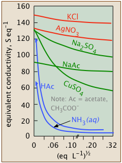
Just as a compact table of thermodynamic data enables us to predict the chemical properties of a very large number of compounds, this compilation of equivalent conductivities of twenty different species yields reliable estimates of the of Λ0 values for five times that number of salts.
Limiting conductivities of weak electrolytes can be estimated
One useful application of Kohlrausch's law is to estimate the limiting equivalent conductivities of weak electrolytes which, as we observed above, cannot be found by extrapolation. Thus for acetic acid CH3COOH ("HAc"), we combine the λ0 values for H3O+ and CH3COO– given in the above table:
Λ0HAc = λ0H+ + λ0Ac–
How fast do ions migrate in solution?
Movement of a migrating ion through the solution is brought about by a force exerted by the applied electric field. This force is proportional to the field strength and to the ionic charge.
Calculations of the frictional drag are based on the premise that the ions are spherical (not always true) and the medium is continuous (never true) as opposed to being composed of discrete molecules. Nevertheless, the results generally seem to be realistic enough to be useful.
According to Newton's law, a constant force exerted on a particle will accelerate it, causing it to move faster and faster unless it is restrained by an opposing force. In the case of electrolytic conductance, the opposing force is frictional drag as the ion makes its way through the medium. The magnitude of this force depends on the radius of the ion and its primary hydration shell, and on the viscosity of the solution.
Eventually these two forces come into balance and the ion assumes a constant average velocity which is reflected in the values of λ0 tabulated in the table above.
The relation between λ0 and the velocity (known as the ionic mobility μ0) is easily derived, but we will skip the details here, and simply present the results:
Anions are conventionally assigned negative μ0 values because they move in opposite directions to the cations; the values shown here are absolute values |μ0|.
Note also that the units are cm/sec per volt/cm, hence the cm2 term.
| cation | H3O+ | NH4+ | K+ | Ba2+ | Ag+ | Ca2+ | Sr2+ | Mg2+ | Na+ | Li+ |
|---|---|---|---|---|---|---|---|---|---|---|
| μ0 | .362 | .0762 | .0762 | .0659 | .0642 | .0616 | .0616 | .0550 | .0520 | .0388 |
| anion | OH– | SO42– | Br– | I– | Cl– | NO3– | ClO3– | CH3COO– | C2H5COO– | C3H7COO– |
| μ0 | .2050 | .0827 | .0812 | .0796 | .0791 | .0740 | .0705 | .0461 | .0424 | .0411 |
As with the limiting conductivities, the trends in the mobilities can be roughly correlated with the charge and size of the ion. (Recall that negative ions tend to be larger than positive ions.)
Cations and anions carry different fractions of the current
In electrolytic conduction, ions having different charge signs move in opposite directions. Conductivity measurements give only the sum of the positive and negative ionic conductivities according to Kohlrausch's law, but they do not reveal how much of the charge is carried by each kind of ion. Unless their mobilities are the same, cations and anions do not contribute equally to the total electric current flowing through the cell.
Recall that an electric current is defined as a flow of electric charges; the current in amperes is the number of coulombs of charge moving through the cell per second. Because ionic solutions contain equal quantities of positive and negative charges, it follows that the current passing through the cell consists of positive charges moving toward the cathode, and negative charges moving toward the anode. But owing to mobility differences, cations and ions do not usually carry identical fractions of the charge.
Transference numbers are often referred to as transport numbers; either term is acceptable in the context of electrochemistry.
Transference or Transport numbers
The fraction of charge carried by a given kind of ion is known as the transference number t±. For a solution of a simple binary salt,

By definition, t+ + t– = 1.
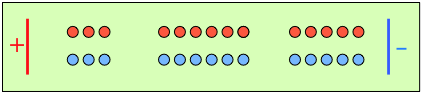
To help you visualize the effects of non-identical transference numbers, consider a solution of M+ X– in which t+ = 0.75 and t– = 0.25. Let the cell be divided into three [imaginary] sections as we examine the distribution of cations and anions at three different stages of current flow.
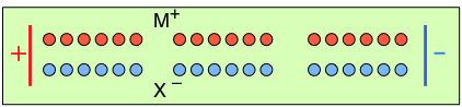 |
Initially, the concentrations of M+ and X– are the same in all parts of the cell. |
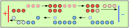 |
After 4 faradays of charge have passed through the cell, 3 eq of cations and 1 eq of anions have crossed any given plane parallel to the electrodes. Note that 3 anions are discharged at the anode, exactly balancing the number of cations discharged at the cathode. |
 |
In the absence of diffusion, the ratio of the ionic concentrations near the electrodes equals the ratio of their transport numbers. |
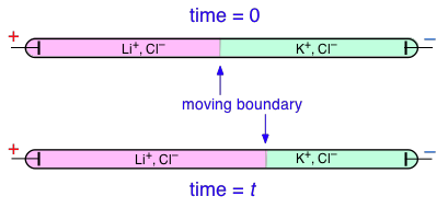
Transference numbers can be determined experimentally by observing the movement of the boundary between electrolyte solutions having an ion in common, such as LiCl and KCl:
H+ and OH– ions "migrate" without moving, and rapidly!
You may have noticed from the tables above that hydrogen- and hydroxide ions have extraordinarily high equivalent conductivities and mobilities. This is a consequence of the fact that unlike other ions which need to bump and nudge their way through the network of hydrogen-bonded water molecules, these ions are participants in this network. By simply changing the H2O partners they hydrogen-bond with, they can migrate "virtually". In effect, what migrates is the hydrogen-bonds, rather than the physical masses of the ions themselves.
This process is known as the Grothuss Mechanism. The shifting of the hydrogen bonds occurs when the rapid thermal motions of adjacent molecules brings a particular pair into a more favorable configuration for hydrogen bonding within the local molecular network.
Bear in mind that what we refer to as "hydrogen ions" H+(aq) are really hydronium ions H3O+, most of which are themselves hydrated, forming units such as H5O2+ and H9O4+. Some theoretical studies suggest that H3O+(H2O)20 might be a major structural form of the "hydronium ion".
It is remarkable that this virtual migration process was proposed by Theodor Grotthuss in 1805 — just five years after the discovery of electrolysis, and he didn't even know the correct formula for water; he thought its structure was H–O–O–H.
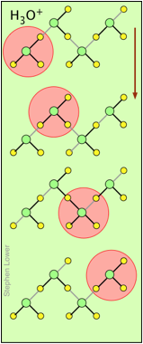
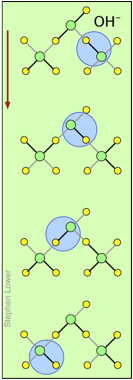
These two diagrams will help you visualize the process. The successive downward rows show the first few "hops" made by the virtual H+ and OH– ions as they move in opposite directions toward the appropriate electrodes. (Of course, the same mechanism is operative in the absence of an external electric field, in which case all of the hops will be in random directions.)
Covalent bonds are represented by black lines, and hydrogen bonds by gray lines.
From the chemist's standpoint, the most important examples of conduction are in connection with electrochemical cells, electrolysis and batteries. These topics are covered in the separate lesson set All About Electrochemistry.
Determination of equilibrium constants by electrolytic conductance
Owing to their high sensitivity, conductance measurements are well adapted to the measurement of equilibrium constants for processes that involve very small ion concentrations. These include
- Ks values for sparingly soluble solids
- Autoprotolysis constants for solvents (such as Kw )
- Acid dissociation constants for weak acids
As long as the ion concentrations are so low, their values can be taken as activities, and limiting equivalent conductivities Λ0 can be used directly.
The ion product of water can be measured by conductance
The very small conductivity of pure water makes it rather difficult to obtain a precise value for Kw; better values are obtained by measuring the potential of an appropriate galvanic cell. But the principle illustrated here might be applicable to other autoprotolytic solvents such as H2SO4.
Use the appropriate limiting molar ionic conductivities to estimate the autoprotolysis constant Kw of water at 25° C. Use the reaction equation
2 H2O → H3O+ + OH–.
Solution:The data we need are λH+ = 349.6 and λOH– = 199.1 S cm2 mol–1.
The conductivity of water is κ = [H+] λH+ + [OH–] λOH– whose units work out to (mol cm–3) (S cm2 mol–1). In order to express the ionic concentrations in molarities, we multiply the cm–3 term by (1 L / 1000 cm–3), yielding
1000 κ = [H+] λH+ + [OH–] λOH– with units S cm–1 L–1.
Recalling that in pure water, [H+] = [OH–] = Kw½, we obtain
1000 κ = (Kw½)(λH+ + λOH– ) = (Kw½)(548.7 S cm2 mol–1).
Solving for Kw: Kw = (1000 κ / 548.7 S cm2 mol–1)2
Substituting Kohlrausch's water conductivity value of 0.043 × 10⁻⁶ S cm–1) for κ gives Kw =(1000 × 0.043 × 10–6 S cm–1 / 548.7 S cm2 mol–1)2
= 0.614 × 10⁻¹⁴ mol2 cm–6 (i.e., mol2 L–2).
The accepted value for the autoprotolysis constant of water at 25° C is
Kw = 1.008 × 10⁻¹⁴ mol2 L–2.
Solubility products can be estimated from limiting ionic conductivities
Conductometric titration
↓ Click on image to enlarge

Conductometric titration setup
A chemical reaction in which there is a significant change in the number or mobilities of ionic species can be followed by monitoring the change in conductance. Many acid-base reactions fall into this category. In conductometric titration, conductometry is employed to detect the end-point of a titration.
Consider, for example, the titration of the strong acid HCl by the strong base NaOH. In ionic terms, the process can be represented as
H+ + Cl– + Na+ + OH– → H2O + Na++ Cl–
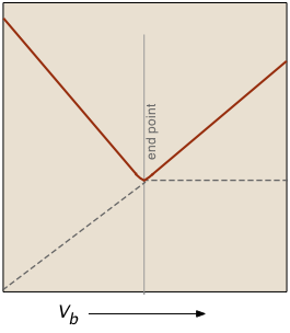
At the end point, only two ionic species remain, compared to the four during the initial stages of the titration, so the conductivity will be at a minimum. Beyond the end point, continued addition of base causes the conductivity to rise again. The very large mobilities of the H+and OH– ions cause the conductivity to rise very sharply on either side of the end point, making it quite easy to locate.
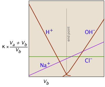
The factor (Va + Vb)/Vb compensates for the dilution of the solution as more base is added.
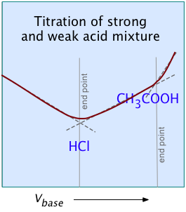
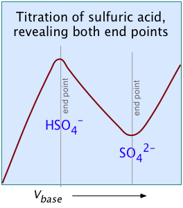
For most ordinary acid-base titrations, conductometry rarely offers any special advantage over regular volumetric analysis or potentiometry. But in some special cases such as those illustrated here, it is the only method capable of yielding useful results.
Electrolytic conduction in the ground
Most people think of electrolytic conduction as something that takes place mainly in batteries, electrochemical plants and in laboratories, but by far the biggest and most important electrolytic system is the earth itself, or at least the thin veneer of soil sediments that coat much of its surface.
Soils are composed of sand and humic solids within which are embedded pore spaces containing gases (air and microbial respiration products) and water. This water, both that which fills the pores as well as that which is adsorbed to soil solids, contains numerous dissolved ions on which soil conductivity mainly depends. These ions include exchangeable cations present on the surfaces of the clay components of soils. Although these electrolyte channels are small and tortuously connected, they are present in huge numbers and offer an abundance of parallel conduction paths, so the ground itself acts as a surprisingly efficient conductor.
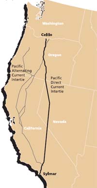
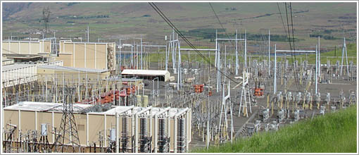
The Celilo Converter Station is located at The Dalles, Oregon
Other applications of ground electrolytic conductance
- Ground-wave radio propagation
- During the daytime, radio transmission at frequencies below about 5 MHz (such as in the old standard AM broadcast band) depends entirely on so-called ground waves that follow the curvature of the earth. This occurs because that portion of the vertically-polarized wave fronts in contact with the earth induce an electrolytic current in the ground, causing their lower portions to travel more slowly, bending their pathways in toward the earth. (See the diagram in this short article on ground-wave propagation.) The U.S Government publishes several ground-conductivity maps that are used to predict the daytime range of AM radio stations in that country.
- Agricultural and environmental soils assessment
- Conductivity has long been used as a tool to assess the salinity of agricultural soils — a serious problem in irrigated regions, where evaporation of irrigation water over the years can raise salinity to levels that can reduce crop yields. Because other soil characteristics (moisture content, density, and mineralogy, fertilization) also play important roles, some care is required to correctly interpret measurements. Measuring devices that can be drawn behind a tractor and are equipped with GPS receivers allow the production of conductivity maps for entire fields.
- Archaeological exploration
- Buried artifacts such as stone walls and foundations and large metallic objects can be located by a series of conductivity measurements at archaeological sites.
